Minimizing the energy of a mechanical structure

This notebook shows how to find the shape of a mechanical structure by minimizing its energy via gradient descent. It illustrates the most powerful function of jax, namely grad.

(C) 2024 Florian Marquardt, Max Planck Institute for the Science of Light (MIT License)

First perform useful imports: matplotlib for plotting, jax.numpy as a replacement for standard numpy, and grad from jax to calculate gradients of functions:

from matplotlib import pyplot as plt
%config InlineBackend.figure_format='retina'

import jax.numpy as jnp
from jax import grad

Defining the energy and taking its gradient

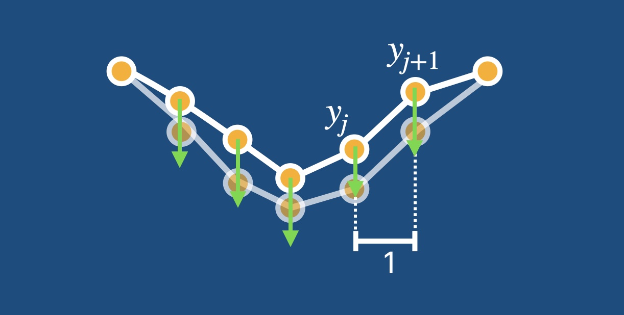
We here define the potential energy of a chain of masses connected by springs. The masses are located at positions that are equally spaced (by 1) in the horizontal direction but located at positions \(y_j\) in the vertical (height) direction. Using Pythagoras, we arrive at:

\[ E = \sum_{j=0}^{N-1} {K \over 2} \left(\sqrt{ (y_{j+1}-y_j)^2 + 1 } - l\right)^2 \]

Here \(K\) is the spring constant, called spring in the following, and \(l\) is the equilibrium length of each spring, called length.

We also add the contribution of a gravitational potential energy:

\[ E_{\rm grav} = \sum_{j=0}^N m g y_j \]

We set \(mg\) to mass_g.

def E(y,spring,length,mass_g):
    """
    Calculate the energy.
    
    y : array containing vertical coordinates, evaluated at x = 0, 1, 2, ...
    spring : spring constant
    length : equilibrium length
    mass_g : mass times g for an individual mass
    """
    
    spring_energy = jnp.sum( 0.5*spring * ( jnp.sqrt((y[1:]-y[:-1])**2 + 1) - length )**2 )
    
    # add contributions from beginning and end (fixed boundaries!):
    spring_energy += 0.5*spring * ( jnp.sqrt(y[0]**2 + 1) - length )**2
    spring_energy += 0.5*spring * ( jnp.sqrt(y[-1]**2 + 1) - length )**2
    
    gravitational_energy = mass_g * jnp.sum(y)
    
    return spring_energy + gravitational_energy
        

Little trick

Since we want to keep the boundaries fixed, at 0 height, we separately added the spring energies of the springs connected to the left and right boundary.

Now we for the first time exploit the power of jax. We simply call grad on the function E, telling it to take the derivative of E with respect to its first argument, which is the array of heights y. This produces a new function, here called grad_E, which has the same arguments as E but now will return the gradient of E with respect to y. Note that this gradient is a vector, while E itself was a scalar function.

# Produce the function that calculates the gradient of E
# with respect to the y argument (argument number 0):

grad_E = grad(E, argnums = 0)

Gradient descent loop

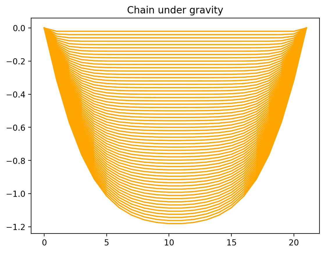
We now perform gradient descent. This means running a loop. In each iteration of this loop we calculate the gradient of E, then subtract it from the current values of the chain shape y, so as to lower the energy, and continue with this process. In order to not make overly large steps, we define a stepsize eta that is multiplied with the gradient before doing the subtraction. Larger stepsizes would result in quicker convergence, but if it gets too large, the process is unstable.

We finally plot all the chain shapes in a single plot, to observe how the chain tries to relax to its equilibrium shape under the influence of both the springs and gravity.

# Physics parameters:
N = 20 # number of masses in the chain
spring = 5.0 # spring constant
length = 0.8 # springs are stretched even when chain is straight!
mass_g = 0.1 # m*g for each mass

# Initialization:
y = jnp.zeros(N) # initially, all masses at y=0

# Now do several steps of gradient descent:

# Gradient descent steps:
nsteps = 60 # number of gradient descent steps
eta = 0.2 # size of each gradient descent step

zero = jnp.array([0.0]) # needed for plotting

for step in range(nsteps):
    y -= eta * grad_E(y, spring, length, mass_g)
    plt.plot(jnp.concatenate([zero,y,zero]), color="orange") # plot with boundaries appended

plt.title("Chain under gravity")
plt.show()

Adaptive-stepsize gradient descent using optax

We are now getting a bit more sophisticated. We will use the optax library to perform gradient descent using an adaptive stepsize. In particular, we will use the famous adam technique which has become a default adaptive-stepsize approach for machine learning.

import optax

Initialize our chain shape and initialize the optimizer that will help us do the adaptive stepsize gradient descent.

# Initialization:
y = jnp.zeros(N) # initially, all masses at y=0

# the gradient step size is called "learning rate"
# in machine learning language:
learning_rate = 0.1

# get the optimizer:
optimizer = optax.adam( learning_rate )
# initialize the 'state' of the optimizer, by
# telling it about the initial values:
opt_state = optimizer.init( y )

Now again do some gradient descent, but using adam. In each step, the gradients grads are calculated, just like before. However, now they are used to calculate the updates using the optimizer, while also updating the internal optimizer state opt_state. This internal state is needed to keep track of things like averages over the size of past gradients, to be able to adapt the gradient stepsize.

# Gradient descent steps:
nsteps = 60 # number of gradient descent steps

zero = jnp.array([0.0])

for step in range(nsteps):
    # get gradients:
    grads = grad_E(y, spring, length, mass_g)
    
    # update y using the gradients:
    updates, opt_state = optimizer.update( grads, opt_state)
    y = optax.apply_updates( y, updates )
    
    plt.plot(jnp.concatenate([zero,y,zero]), color="orange") # plot with boundaries appended

plt.title("Chain under gravity")
plt.show()

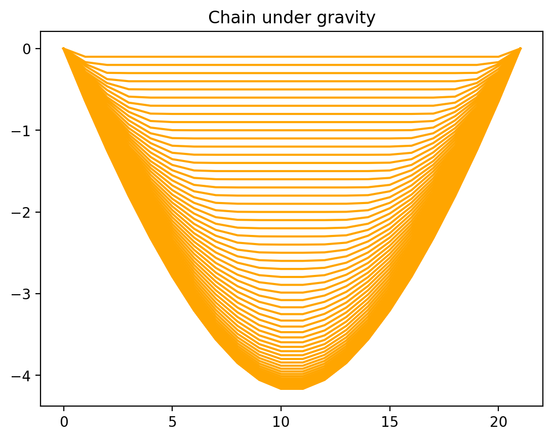
We see that in the same number of steps, the chain is now actually converged to its final equilibrium shape, which was not yet the case before!

Exercise

If you are interested in playing with the physics of this example, try changing the equilibrium spring length and run the gradient descent again (interesting values are 1 and also values above 1).

Outlook

optax offers many more choices for the optimizer beyond “adam”. In addition, it allows useful things like changing the overall stepsize (or “learning rate”) as a function of time.